This post is a (non-exhaustive) summary of the techniques I’ve used to accelerate neural network training. I’m going to focus on the most fundamental adaptations to improve the training process, excluding the obvious SIMD/multicore/parallelism/memory/hardware techniques, which I may cover later in a separate post. Realistically, this post is only a snapshot in time: some of the techniques I talk about will likely become obsolete in the next few years as newer, better training optimizations are discovered. But that’s okay! I’ll still (hopefully) be around to write about them.
Preconditioning
The goal: rescale the weight space so the level sets are circular.
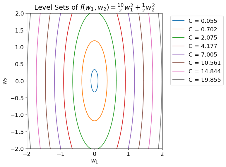
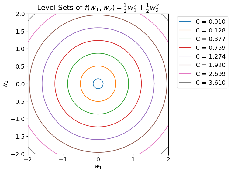
Learning is fundamentally an optimization problem. Our goal is to optimize the model’s weights to minimize the loss, so it’s useful to think about how difficult this optimization problem is. One metric for “difficulty” is the condition number, \(\kappa\). When \(\kappa\) is large, it means our problem is difficult and will take many iterations of gradient descent to find a local minimum. Intuitively, \(\kappa\) hints toward how complex the underlying space we’re trying to optimize is. The goal of preconditioning is to lower \(\kappa\) for our problem so the space we’re optimizing is smooth. In practice we do this by scaling the gradients we compute when performing gradient descent. That is, instead of our weight update being \(w_{t+1} = w_t - \alpha \nabla f(w_t)\) it’s \(w_{t+1} = w_t - \alpha P \nabla f(w_t)\) where \(P\) is a positive semidefinite matrix. If our model is large, then \(P\) will be too, since \(P\) will be a \(d^2\) matrix where \(d\) is the number of weights in our model. So how do we choose \(P\) so that it rescales our underlying weight space and isn’t too computationally expensive? One way is to use a diagonal approximation of Newton’s method. [1] Generally, this is still pretty expensive, which is why preconditioning isn’t usually anyone’s first thought when trying to speed up training.
Batch Normalization
BatchNorm is one of the most widely used optimization techniques, because it works well and is easy to implement. The inventors of BatchNorm, Sergey Ioffe and Christian Szegedy, saw a problem with the way deep neural networks were trained. Because the inputs to each layer are affected by the parameters of all earlier layers, small perturbations upstream will amplify as the signal moves through the network. That means that later layers will experience a constant shift of the underlying optimization problem, making training difficult. The authors named this problem internal covariate shift, and formalized it as “the change in the distribution of network activations due to the change in network parameters during training.” [2] To fix this problem, they developed BatchNorm. BatchNorm operates on batches (duh) of input to each layer. Let’s say the input to some layer is a tensor \(x \in R^d\). BatchNorm takes a batch of training inputs and normalizes them using the mean and variance of the batch, e.g. for some input \(x_i\), \(\hat{x_i} = \frac{x_i - \mu_B}{\sqrt{\sigma^{2}_B + \epsilon}}\) where \(\epsilon\) is some small value to avoid division by zero and \(\mu_B\) and \(\sigma_B\) denote the mean and variance of the batch. But! This normalization might change what the layer can actually represent, which defeats the purpose. So to ensure that our transformation (normalization) can represent the identity transform, we add two learnable parameters \(\gamma\) and \(\beta\) to scale and shift the normalized value. Our final output is then \(\text{BatchNorm}(x_i) = \gamma \hat{x_i} + \beta\). If you’re confused about \(\gamma\) and \(\beta\), good! When we normalized our input, we set the mean and standard deviation to \(0\) and \(1\); however, that isn’t really what we wanted to do. We wanted to eliminate the current layer’s dependency on previous layers’ parameters, and we’ve done that by replacing all those complex dependencies with just two parameters, \(\gamma\) and \(\beta\). It’s much easier to learn two parameters (for each BatchNorm layer) than to learn some complicated interaction between previous layers’ parameters. At inference time, since we aren’t using batches, we can’t calculate a mean and variance of each batch. Instead we just replace \(\mu_B\) and \(\sigma_B\) with \(\mu_{\text{Dataset}}\) and \(\sigma_{\text{Dataset}}\) when computing \(\hat{x_i}\).
Unfortunately, BatchNorm doesn’t actually do what the authors thought it would do, but that wasn’t discovered until a few years later. To be clear, I don’t mean that BatchNorm doesn’t work. It does! The authors just didn’t understand the mechanism behind why it works. It’s most likely that BatchNorm doesn’t actually decrease internal covariate shift (in fact, it may increase it in certain cases) but instead conditions the loss landscape to be more Lipschitz-smooth. [3] This means that BatchNorm is performing a similar function to preconditioning, given that Lipschitz-smoothness is similar to condition number because it provides a bound on how quickly the gradients in your loss landscape can change. Regardless of how it operates, BatchNorm can greatly decrease the amount of time it takes training to converge.
Layer Normalization
Batch normalization achieved overnight popularity, but it had its problems. First, BatchNorm can’t be used with recurrent architectures because the mean and variance computed for each batch would transcend time steps–this meant it couldn’t be used in RNNs and LSTMs. In addition, BatchNorm had another problem that affected large-scale non-recurrent networks: the choice of batch size. Since BatchNorm is dependent on the size of the batch, massive datasets would require large batch sizes to produce representative \(\mu_B\) and \(\sigma_B\), and this makes distributed learning challenging. Layer normalization remedies both of these challengesby transposing BatchNorm. In BatchNorm, we normalized the input to each neuron using the mean and variance of a batch of inputs. LayerNorm takes a single input and normalizes the input using the mean and variance of activation to each neuron in the layer. Like BatchNorm, LayerNorm introduces two parameters to scale and shift the normalized input. However, unlike BatchNorm, there is no difference between LayerNorm at train time and inference time–LayerNorm always performs the same transformation.
Should I always use LayerNorm instead of BatchNorm?
Well… no. LayerNorm is the clear choice for recurrent architectures, because BatchNorm averages across hidden state time steps; however, it seems that LayerNorm sometimes performs poorly on convolutional architectures, although not always. The original LayerNorm paper found lackluster performance in convolutional networks, stating “further research is needed to make layer normalization work well in ConvNets.” [4] However, other researchers have found that LayerNorm can sometimes outperform BatchNorm in ConvNets, but sometimes doesn’t. [5]
Optimizer choice
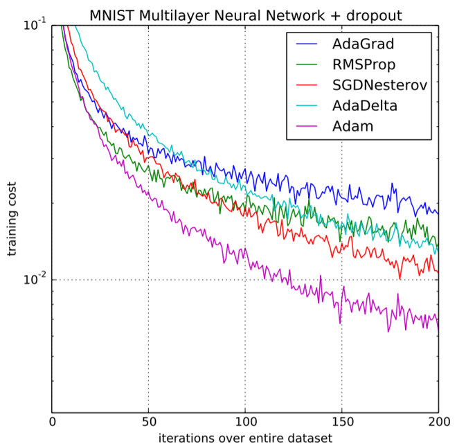
The choice of optimizer has a huge impact on both how quickly your network can converge to a small loss value. Nowadays, all of the “serious” optimizers use a different learning rate for each parameter. I’ve nearly always used Adam or AdamW in practice, but since they’re built on RMSProp and AdaGrad, I’ve included short descriptions of each. There are dozens of other optimizers, but these are the basics.
AdaGrad
AdaGrad keeps track of the weighted sum of each parameter’s gradient during gradient descent. The step size for each parameter is then inversely proportional to the square root of the parameter’s all-iterations-sum. This works well for convex settings, but neural networks are not convex. Since the learning rate for each parameter is dependent on the entire history of its gradient, we could be optimizing through terrain of extremely different curvature than we previously were, making our step size inappropriate.
RMSProp
This approach built on AdaGrad and attempted to fix its shortcoming. Instead of keeping track of the entire history of gradients, RMSProp uses an exponential moving average rather than a sum. One problem with RMSProp is that the exponential average is initialized to zero, which may bias the learning rates, particularly in the first few iterations.
Adam
Adam combines RMSProp with momentum. Momentum looks at the sign of the gradient for each parameter. The idea is that if the sign of a parameter’s gradient flips between iterations, then that parameter stepped too far and its learning rate should be decreased. If the sign doesn’t flip, then we can take a bigger step and increase the learning rate. There are different types of momentum, but that’s enough to understand how it works for Adam. One final difference between Adam and RMSProp is that Adam includes a bias correction terms to reduce the bias caused by initializing the moving average to zero.
AdamW
I’ve never personally noted a difference in training with AdamW as opposed to Adam, but that doesn’t mean it’s the case for every network. AdamW is actually the correct implementation of Adam, which major ML frameworks like PyTorch, JAX, and TensorFlow had implemented slightly incorrectly. The AdamW implementation decouples weight decay \(\beta\) from learning rate \(\alpha\). It’s a very slight implementation difference, but might result in better performance.[6]
An Important Note about Initialization
Initialization is often overlooked, but a poor initialization can drastically increase the number of epochs needed to train a model. In some cases, the wrong initialization can prevent the model from learning at all. The two most well-known initialization strategies are Xavier initialization and He initialization (also sometimes called Kaiming initialization).
Xavier Initialization
This form of initialization was designed to mitigate the exploding/vanishing gradient problems. The original paper specifies that the weights for layer \(i\) should be drawn from \(U[-\frac{\sqrt{6}}{\sqrt{N_i + N_{i + 1}}}, \frac{\sqrt{6}}{\sqrt{N_i + N_{i + 1}}}]\), where \(N_i\) is the number of connections to layer \(i\). The paper doesn’t actually justify the use of the uniform distribution; instead, the important feature of Xavier initialization is that the weights should be drawn from some distribution centered at zero, with a variance of \(\frac{1}{N_i}\). [7]
He Initialization
Xavier initialization worked great with sigmoid and tanh activation functions. Unfortunately, it’s been shown to sometimes stymie learning in networks with ReLU or ReLU variant activations. He initialization rectifies this (pun intended) by using a larger variance of \(\frac{2}{N_i}\). The authors decided to use a normal distribution instead of a uniform distribution, but again, they didn’t make any claims about the distribution, just the variance. [8]
Now, The Interesting Part..
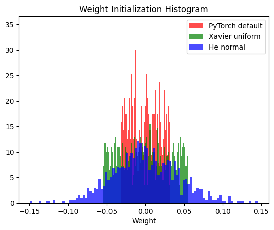
For a long time I assumed that ML frameworks like PyTorch would default initialize model weights according to the activation type. For some reason, PyTorch does not default initialize model weights using Xavier or He. Instead, linear layers are initialized from \(U[-\frac{1}{\sqrt{N_i}}, \frac{1}{\sqrt{N_i}}]\). I haven’t yet found any justification for why this initialization is used as opposed to Xavier or He, both of which are implemented and can be manually selected for initialization. Here’s a histogram showing how the weights compare for the same model using Xavier init, He init, and PyTorch’s default init.
Out of curiosity, I decided to compare performance of a model using various initialization strategies on the MNIST dataset. For this experiment, my model had three linear layers with ReLU activations and used Adam with a batch size of 128 and a very low learning rate of \(0.0001\). The code for this experiment is posted here.
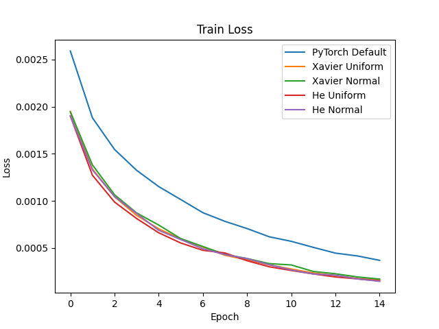
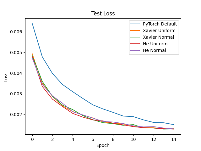
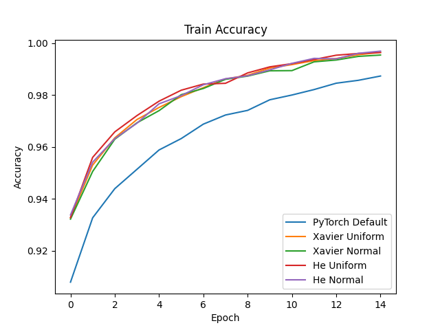
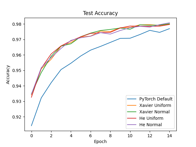
Clearly, Xavier and He initialization far outperform PyTorch’s default weight initialization! Also noteworthy is that, at least in this experiment, Xavier and He resulted in equal performance. In addition, it made no difference whether the initialization type used a uniform or normal distribution, which is expected given that Xavier and He both only make claims about the variance of the distribution, not the distribution type. The key takeaway: never trust the default settings of your ML framework. Explicitly initialize your model’s weights!
References
I’ve only given rough summaries of these techniques, covering the details that I find most important in my experience. For a more in-depth explanation, look at the resources here.
[1] Newton Sketch: A Linear-time Optimization Algorithm with Linear-Quadratic Convergence
[2] Batch Normalization: Accelerating Deep Network Training by Reducing Internal Covariate Shift
[3] How does Batch Normalization Help Optimization?
[6] Decoupled Weight Decay Regularization
[7] Understanding the difficulty of training deep feedforward neural networks
[8] Delving Deep into Rectifiers: Surpassing Human-Level Performance on ImageNet Classification