
When we think about solving problems using machine learning, usually our first concern is building a model that is good at whatever it is we want it to do. For object detection systems, we first want to ensure our model is good at detecting objects. For machine translation tasks, we want to ensure our model accurately translates among languages. But usually we also have other constraints for our machine learning task, such as latency, memory limitations, or how much we’re willing to spend on cloud compute. One way we can address each of these issues is through model compression and quantization. I’m going to survey a few of the ways neural networks are currently being compressed, and I’ll end with a look at what’s up-and-coming.
Quantization
“Why waste time memory use many word bits when few word bits do trick?” –Kevin, from The Office, on quantization

Quantization cuts down the size of our model by targeting the number of bits used to represent floating point numbers. If every weight in our model is a float with \(x\) bits, and we replace each weight with an equivalent representation that only has \(\frac{x}{2}\) bits, then we’ve cut the memory requirement of our model in half. Unfortunately, there is no free lunch, and we can’t just replace all single precision (\(32\) bit) floating point numbers with half precision (\(16\) bit) floats and call it a day. Reducing the number of bits comes at the cost of range, precision, or both. Let’s look at the IEEE format for a \(32\) bit floating point number.
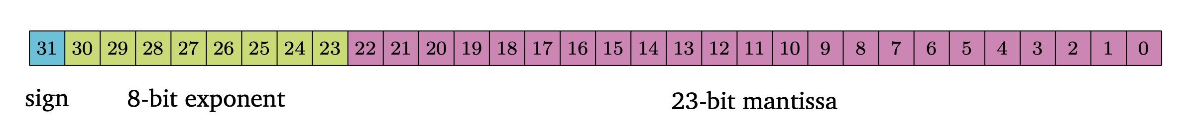
We see that one bit is reserved to determine the sign of the number. Another \(8\) bits are reserved for the exponent, and \(23\) for the mantissa. The human-readable number we represent is given by \((-1)^{\text{sign}} \cdot 2^{\text{exponent} - 127} \cdot 1.\text{mantissa}\) where \(\text{exponent}\) is the decimal representation of the exponent bits and mantissa sums the values of the mantissa where \(b_{22} = \frac{1}{2}\), \(b_{21} = \frac{1}{4}\), \(b_{20} = \frac{1}{8}\), etc. There are a few special cases (\(\pm \infty\), NaN, denormal numbers) that I won’t describe here, but what we can see from the representation is that the range of the float is mostly determined by the exponent bits, while the precision of the number is determined by the mantissa bits. When I say precision, I’m specifically talking about a value called machine epsilon, \(\epsilon\). \(\epsilon\) bounds the maximum error that a floating point representation can have when representing any real number within that float’s range. Again, I’m ignoring some things like overflow, denormals, and invalid computations, but this isn’t a course in computer systems. Armed with our knowledge of \(\epsilon\), let’s return to the IEEE single precision float. If we remove some of the mantissa bits, our \(\epsilon\) increases–meaning we won’t be able to represent numbers as precisely. If we remove some of the exponent bits, then we decrease the range of numbers that we can represent, which makes us more likely to have overflow. So what do we do? As it turns out, in machine learning we really don’t care that much about precision. The extent to which we don’t care is currently up for debate, but for now it’s been shown that \(7\) mantissa bits is generally precise enough for machine learning. That leads us to the bfloat16, a \(16\) bit floating point format with the same range as IEEE \(32\) bit floats, at the cost of a higher \(\epsilon\).
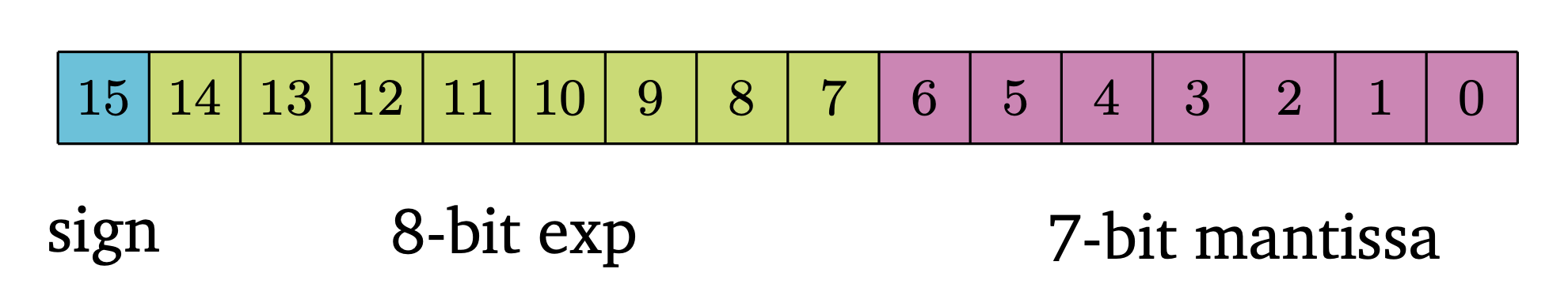
Notice that the bfloat16 (b for “brain” as in Google Brain) has the same number of exponent bits as the IEEE single precision float. This is in contrast to the IEEE half precision float, which has fewer exponent bits and thus a smaller range. Because of this, you can use bfloat16 pretty much anywhere you previously used single precision floats, with no need to change any hyperparameters. [1] [2] [3] Memory isn’t the only benefit of using bfloat16. I told a monkey to build and train a small model on the MNIST dataset to compare the performance of double precision, single precision, and bfloat16 formats.
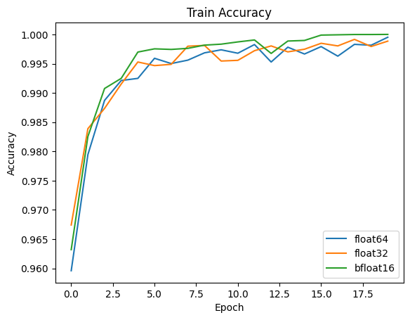
In this example, we can see the model accuracy is the same for all float formats. In addition, I measured the size of the model’s weights and the time it took to train.
| Format | Memory (MB) | Train Time (s) |
|---|---|---|
| float64 | 77.3 | 28 |
| float32 | 38.8 | 22 |
| bfloat16 | 19.1 | 12 |
Clearly the model’s memory footprint is cut in half as we move to lower precision formats. We can also see that training took less time as the size of our floating point format decreased. So how does memory affect training speed?
One possible way memory can affect training speed is if our system is constrained by memory bandwidth. That is, the limiting factor isn’t how fast we can compute a matrix multiply, it’s how quickly we can load data from memory into our processor. Using bfloat16 means we can fit effectively twice as much data into our faster caches, which may reduce or eliminate our bandwidth constraint. Another factor that affects speed is density. In silicon design smaller \(=\) faster, and hardware multipliers (the part that performs multiplications) increase in size proportional to the length of \((\text{mantissa})^2\)! This means that hardware designed with bfloat16 in mind can pack much more circuitry into a smaller area, increasing speed.
Mixed Precision
Hardware today is being built with bfloat16 in mind, such as Nvidia A100 GPUs, Google TPUs, and Apple M2 chips. For now, bfloat16 is usually used to train neural networks in mixed precision. Mixed precision allows training with bfloat16 weights, gradients, and activation values, while optimizer states and a master copy of the weights are single precision format. Current hardware supporting bfloat16 uses \(16\) bit fused multiply-and-accumulate (FMAC) compute units. These FMAC units are designed to compute \(a \leftarrow a + x \cdot y\) where \(x\) and \(y\) are input float numbers and \(a\) is a \(32\) bit accumulator. Since the accumulator is \(32\) bits, the output of the FMAC unit has to be rounded to bfloat16 format. [4] I would not be surprised at all if training using only bfloat16 formats (weights, gradients, optimizer states all stored in bfloat16, accumulator rounding using something like stochastic rounding) takes over in the nearish future. [5]
Pruning
Pruning is another simple way to reduce model size by getting rid of activations that aren’t really contributing much to our model. A simple heuristic that implements this is to prune (remove) the smallest \(x\)% of weights in our model. In practice, we usually “remove” weights by setting them to zero before converting weight matrices to Compressed Sparse Row or Compressed Sparse Column form. Even though we only prune small weights, this still can change how the model behaves, so usually pruning is used hand-in-hand with fine-tuning. Fine-tuning just retrains the network’s non-pruned weights for a small number of epochs at a low learning rate to try to recover some accuracy that might have been lost as a result of pruning. We can even iteratively prune then fine-tune, and models that are trained in this way can be compressed ridiculously small without sacrificing accuracy. Fortunately, it’s not really necessary to implement pruning from scratch. Most ML frameworks have some feature to facilitate model pruning (torch.nn.utils.prune in PyTorch), but you can also extend these features to implement pruning based on your own custom pruning heuristic (PyTorch: subclass BasePruningMethod).
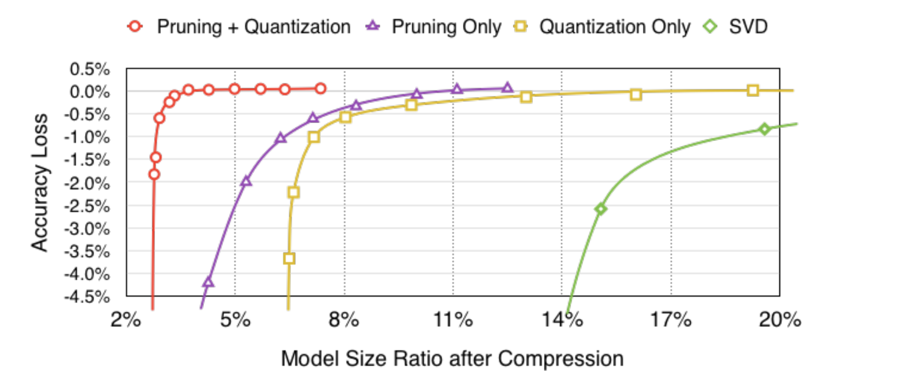
One final interesting bit about pruning: it turns out that pruning followed by quantization produces a more accurate model than just pruning or just quantization. This means that if you want a model that’s as small as possible, your best bet is to use a combination of these techniques. [6]
Distillation
“Machines making training machines! How perverse.” –C-3PO, on distillation

In distillation, we train a large neural network (or even an ensemble of large networks) and then distill the knowledge into a much smaller neural network, usually in situations where we want to deploy our model on edge devices which demand fast inference speeds and have tight memory constraints. The large model (teacher) provides soft targets (class probability distributions) to the small model (learner) for training. The loss function of the learner usually takes into account both the predicted class label and the cross-entropy between the learner’s soft targets and teacher’s soft targets. The original distillation paper used a weighted average of these two objectives, in addition to using an elevated temperature for both the teacher and learner’s soft targets. [7] Distillation works really well, and many of the edge ML applications we use on a daily basis rely on it. For example, Apple used distillation to train the model that performs face detection on iPhones. Interestingly, distillation can sometimes result in a smaller model with higher accuracy than the teacher model. So not only can your distilled model be smaller and faster, it may also be more accurate!

The future
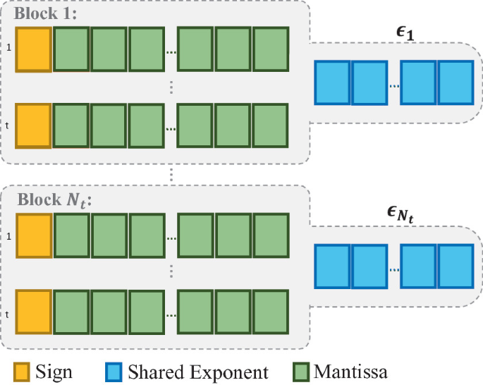
As ML moves into edge devices, there’s a growing need for smaller, faster models that use less power. Model compression is a huge area of research right now, and the methods above only skim the surface. In addition to edge devices, LLMs are ripe for quantization since they contain billions of parameters. One new approach uses clever rounding to quantize LLMs to just two bits post-training. [8] Other compression schemes include block floating point, where a vector of similarly valued floats is stored with a shared exponent and individual mantissas. [9]
Block floating point
In addition, there’s fixed point as an alternative to floating point. This idea is an old one that’s never really taken off in ML (though it certainly has in gaming). The problem right now is a lack of hardware support for low precision fixed point arithmetic such as \(4\) bit operations, which is where fixed point would shine. In all these approaches, the bottleneck right now is hardware. But as we saw with the bfloat16, if something works well it doesn’t take long for the industry to develop hardware that supports it.
References
[1] A Study of BFLOAT16 for Deep Learning Training
[2] BFloat16: The secret to high performance on Cloud TPUs
[3] The bfloat16 numerical format
[5] Revisiting BFloat16 Training
[7] Distilling the Knowledge in a Neural Network
[8] QuIP: 2-Bit Quantization of Large Language Models With Guarantees
[9] FAST: DNN Training Under Variable Precision Block Floating Point with Stochastic Rounding