Neural networks have taken over ML, and I don’t see that changing in the near-term. With everyone focused on transformers and generative AI, it’s worthwhile to take a step back and examine some situations where neural networks aren’t the right tool for the job. There are (sometimes) easier tools to use that work just as well yet offer faster inference speeds and much lower training times. These are my top picks for classification and regression tasks without neural networks.
k-Nearest Neighbors
The benefit of k-NN is that it works well with small, low-dimensional datasets and has zero training time. This is pretty much the first algorithm covered in an introductory ML course (it was in mine!) because it’s so simple. We store all of our training data as vectors, and use some distance function to compare all training data to our test point. We take the mode (or average, if doing regression) of the k closest points to our test point and assign that label to our test point. The important things to note:
- k-NN results depend on the choice of distance function. Usually Minkowski distance is used \(\text{dist}(x, z) = (\sum_{i=1}^{d} \lvert x_i - z_i\rvert^p)^{\frac{1}{p}}\)
- The time complexity of k-NN inference is \(O(n(d+k))\) and memory is \(O(nd)\) where \(d\) is the dimensionality of the data
Speaking of dimensionality, k-NN suffers from the curse of dimensionality. Because distance loses meaning as dimensionality increases and everything becomes very spread out, our k-NN assumption (that a test point will have the same label as the points closest to it) breaks down. So although it is a really simple algorithm, it isn’t practical for high-dimensional data or large datasets because of the curse of dimensionality and inference speed depending on \(n\).
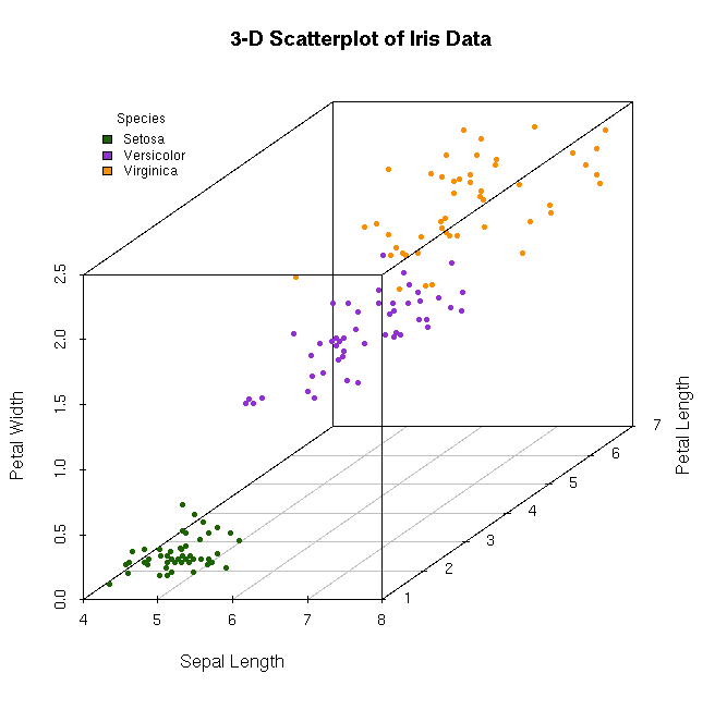
Ideal for k-NN: Iris, with 4 dimensions and 150 data points
Support Vector Machine
Like k-NN, SVMs can be useful when there is very limited data; however, unlike k-NN, they are also able to work with higher dimensional data. Unfortunately, I think the writing is on the wall for SVMs, but they at least deserve a mention before neural networks relegate them to the past. The goal of a Support Vector Machine is to linearly separate data while maximizing the distance from the separating hyperplane to each class. There’s a lot of cool math (kernel tricks, soft constraints, etc) that I’m not going to get into, because I really think SVMs will soon be left in the past. However, if you find k-NN and SVMs interesting, Large Margin Nearest Neighbor classifiers are what happens when k-NN and SVM make a baby. [1]
Classification And Regression Trees (CART)
The main benefit of CART is its interpretability and fast inference. Like k-NN, CART is useful with low dimensional data. Rather than store all the training data and compare it to the test point at inference time, CART uses the data to build a tree structure that recursively divides the space into subspaces with the same label (or, in the case of regression, similar labels). To “train” the algorithm, we take our dataset of \(n\) points and cut the subspace spanned by the data in half. We try splitting at each data point and at each dimension to find which split minimizes some impurity function (maximizes the homogeneity of points on each side of the split). We then continue recursively, performing the same procedure on each side of the split. Usually the algorithm terminates once all labels in subspace are the same or there are no more attributes that can split the data of a subspace. Additionally, we can force the algorithm to stop prematurely (and avoid overfitting!) by specifying a maximum tree depth. Once our tree has been built, we perform inference by traversing down the tree to a leaf node. If our task is classification, the leaf value holds the mode of training data within its subspace (or mean value, in the case of regression).
Example of a Simple CART Tree

Clearly CART is very transparent and interpretable, unlike most ML algorithms. But what are its drawbacks? Since there are \(n\) data points and \(d\) dimensions, we actually have to check \(nd\) potential splits each time. This leads to an average training time complexity of \(O(nd \cdot \text{log}(n))\) and a worst case \(O(n^2d)\). At inference time, all we need to do is traverse down a tree, which is logarithmic in the height of the tree. This means inference is fast. Unfortunately, CART is extremely prone to overfitting, which is why we usually specify a maximum depth. There are other methods to make CART effective, however…
Ensemble Methods
Ever heard the saying “you can’t polish a turd”? It isn’t always true, and that’s kind of the idea behind ensemble methods. We take poorly performing models, lump them together, and the result is a model that works.
Bagging (Random Forest)
The Weak Law of Large Numbers says that for IID random variables \(x_i\) with mean \(\bar{x}\), \(\frac{1}{m}\sum^{m}_{i=1} x_i \rightarrow \bar{x}\) as \(m \rightarrow \infty\). So let’s apply this to ML. Let’s assume an oracle gave us access to a bunch of datasets \(\mathcal{D_1}, \mathcal{D_2}, .., \mathcal{D_m}\) drawn from the true distribution. If we train a model on each of these datasets and average their predictions, we’ll get a model that behaves as if it was trained on the true distribution (has no variance). In math, that’s \(\frac{1}{m}\sum^{m}_{i=1} h_{\mathcal{D_i}} \rightarrow \bar{h}\) as \(m \rightarrow \infty\) where \(\bar{h}\) is the unattainable model with no variance. But we only have one dataset, \(\mathcal{D}\), and we don’t have an oracle who can hand us datasets drawn from the true distribution (if we did, ML would be pretty easy). Instead, we can simulate these datasets by drawing from \(\mathcal{D}\) with replacement. If this sounds a little handwavy, it’s because it is. The Weak Law of Large Numbers doesn’t hold for our simulated datasets—but, in practice this still reduces the variance. This approach is called bagging and is very effective when you have the resources to quickly average many high-variance (overfitting) models. We saw in our discussion of CART that it quickly overfits, so we can use a bagging algorithm called Random Forest.
Some Random Forest I found on the Internet

In this algorithm, we sample \(m\) datasets from \(\mathcal{D}\) with replacement and train a decision tree on each dataset. We slightly modify the CART process to increase the variance: we train each tree to max depth, and with each split we only consider a random subset \(k\) of our \(d\) features. To get a prediction, we just compute the average of our \(m\) trees. Random Forest is just about the easiest ML algorithm you can use, because there are only two hyperparameters, \(m\) and \(k\), and they’re both easy to set. Typically \(k = \sqrt{d}\) works well for classification tasks, and \(k=\frac{d}{3}\) is good for regression. Obviously, the variance will decrease as we increase \(m\); however, this will also slow down inference, since we will need to traverse down \(m\) trees to make a prediction. So your choice of \(m\) is a tradeoff: do you value slightly higher accuracy, or faster inference speeds? One final note about choosing \(m\)—it’s very easy to parallelize. Each tree can be traversed on its own core, so use that to speed up inference with many trees!
Boosting
With bagging, we averaged many high variance models to produce a model with low variance. Boosting iteratively combines high bias models to produce an aggregate model that has lower bias. It is closely related to gradient descent, and even uses our classic \(\alpha\) learning rate hyperparameter! At each iteration we combine a high bias model \(h\) with our aggregate model \(H\) such that our loss \(\ell(H) = \frac{1}{n}\sum^{n}_{i=1} \ell(H(x_i), y_i)\) decreases with each iteration. So at each iteration \(t\), we choose a model \(h_{t+1} = \text{argmin}_{h \in \mathbb{H}} \ell(H_t + \alpha h_t)\) and combine it with \(H\). There are many different boosting algorithms, including LogitBoost, Gradient Boosted Regression Trees, and AdaBoost (which uses an adaptive \(\alpha\)).
References
[1] Distance Metric Learning for Large Margin Nearest Neighbor Classification